WK05
Intro to GIS / Spatial Data
GIS, or the social construction of spatial data — a map is an argument about the world, not the world
GIS — or the Social Construction of Spatial Data
LAAR 61400 · Week 05
Part I

A map is an argument

Part II

From globe to grid

Part III

How space becomes data

Part IV

Analysis

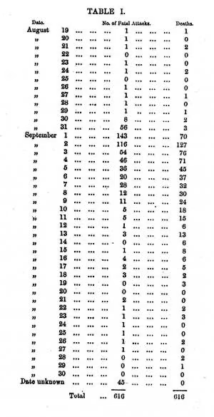
Table of London cholera mortality, 1854
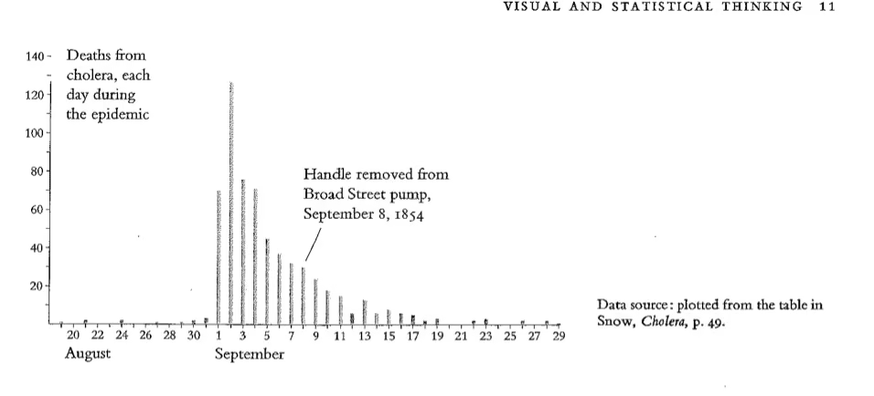
Cholera deaths plotted over time as a bar chart
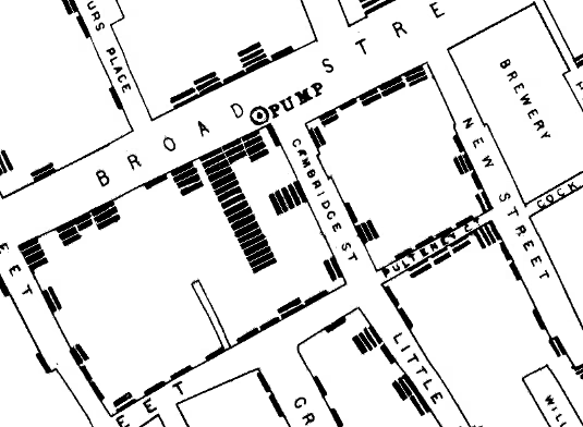
John Snow cholera map, detail
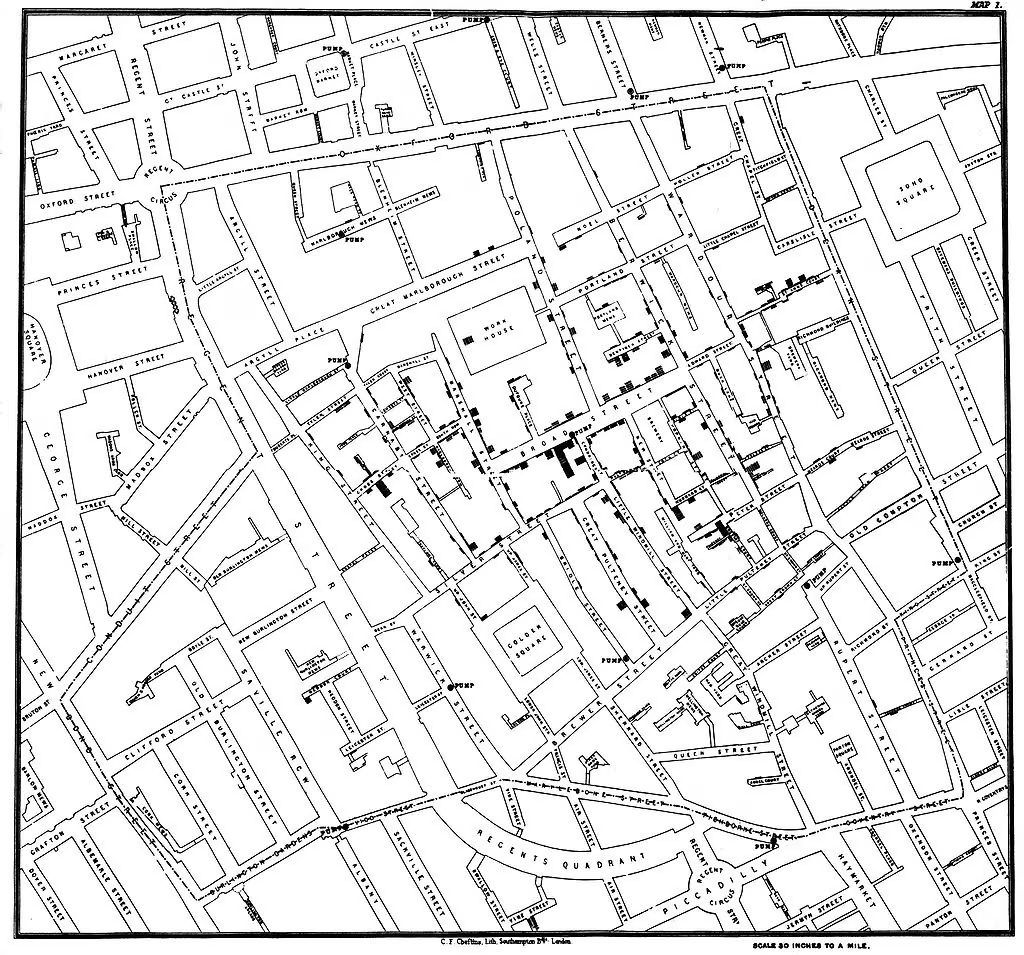
John Snow cholera map, full
“Science manipulates things and gives up living in them. Constructive scientific activities see themselves and represent themselves to be autonomous, and their thinking deliberately reduces itself to a set of data-collecting techniques which it has invented. To think is thus to test out, to operate, to transform—the only restriction being that this activity is regulated by an experimental control that admits only the most "worked-up" phenomena, more likely produced by the apparatus than recorded by it.”
Maurice Merleau-Ponty · Eye and Mind · 1961
Part I

A map is an argument

Part II

From globe to grid

Part III

How space becomes data

Part IV

Analysis

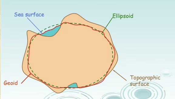
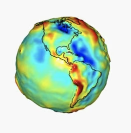
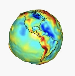
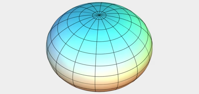
The geoid — exaggerated gravity-field surface of the earth
Geoid undulation globe
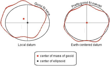
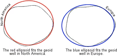
A spheroid fitted to the geoid
Datum reference — NAD27 vs NAD83
Geographic coordinate system globe
Latitude and longitude graticule on a globe
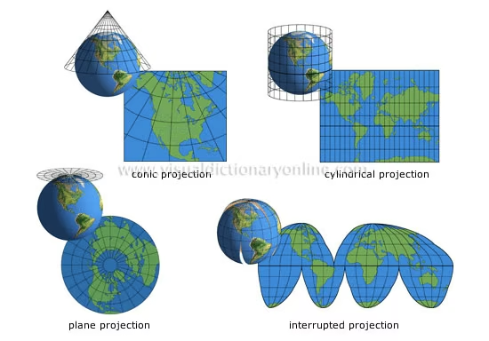
Projecting the spheroid onto a flat plane
Conic, cylindrical and planar developable surfaces
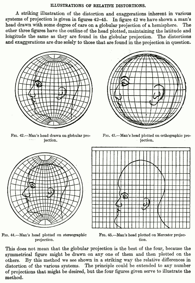
A face projected onto a globe and back — distortion illustration
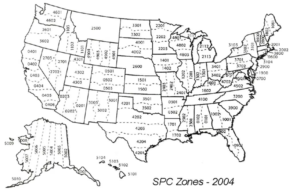
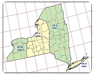
US State Plane Coordinate zones map
State Plane zone detail
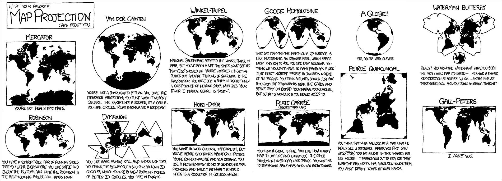
A grid of different world map projections
Part I

A map is an argument

Part II

From globe to grid

Part III

How space becomes data

Part IV

Analysis

RASTERvsVECTOR

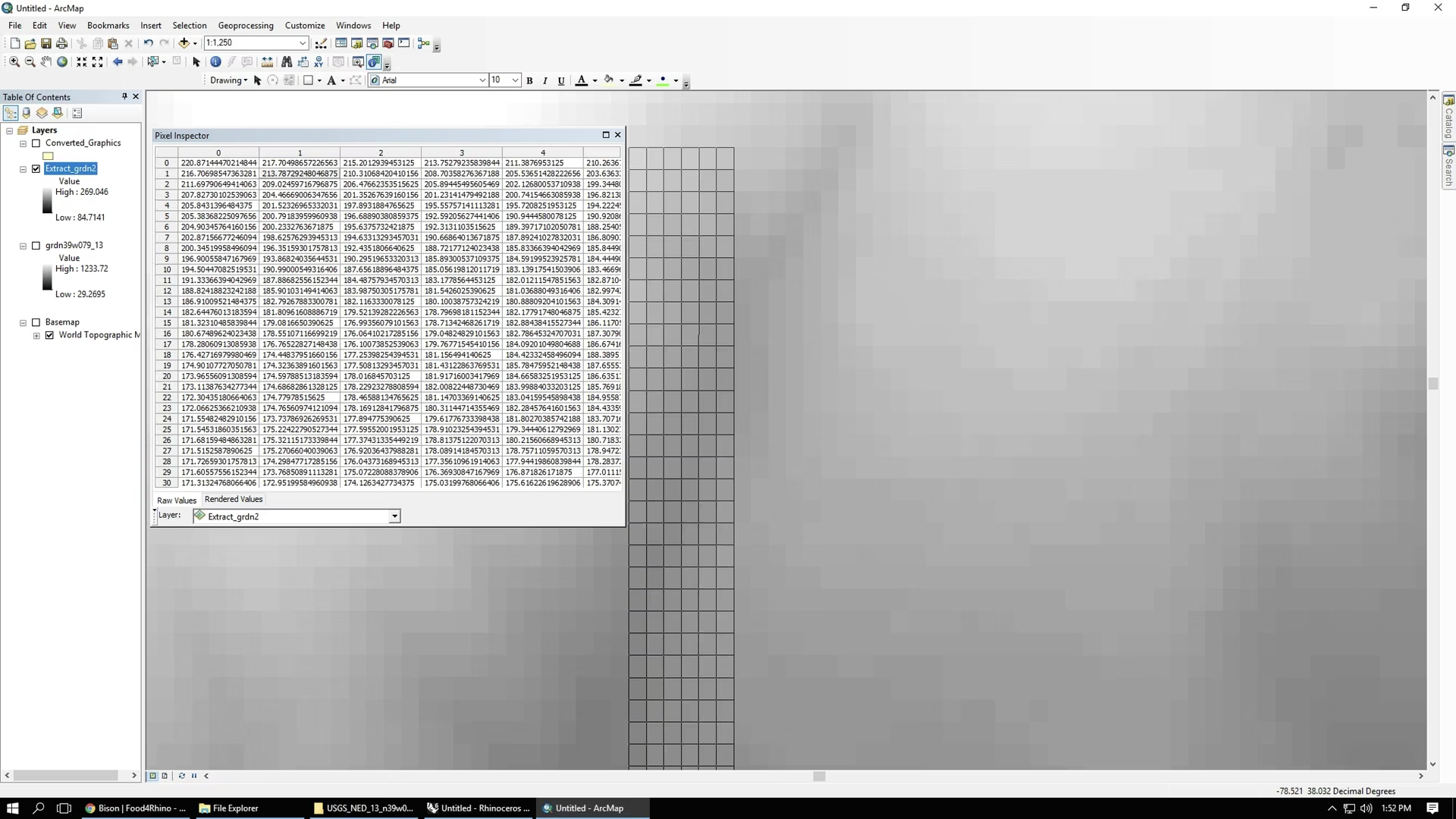
Vector stores objects with edges — points, lines, polygons. Raster stores a field sampled on a grid of cells. The model you pick pre-decides which questions are easy.

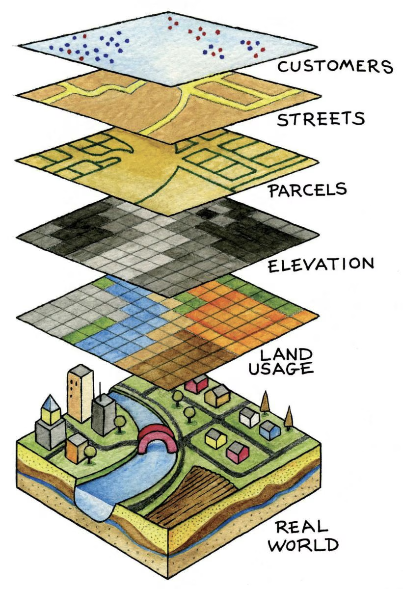
GIS layers stacked: elevation, land use, parcels, streets
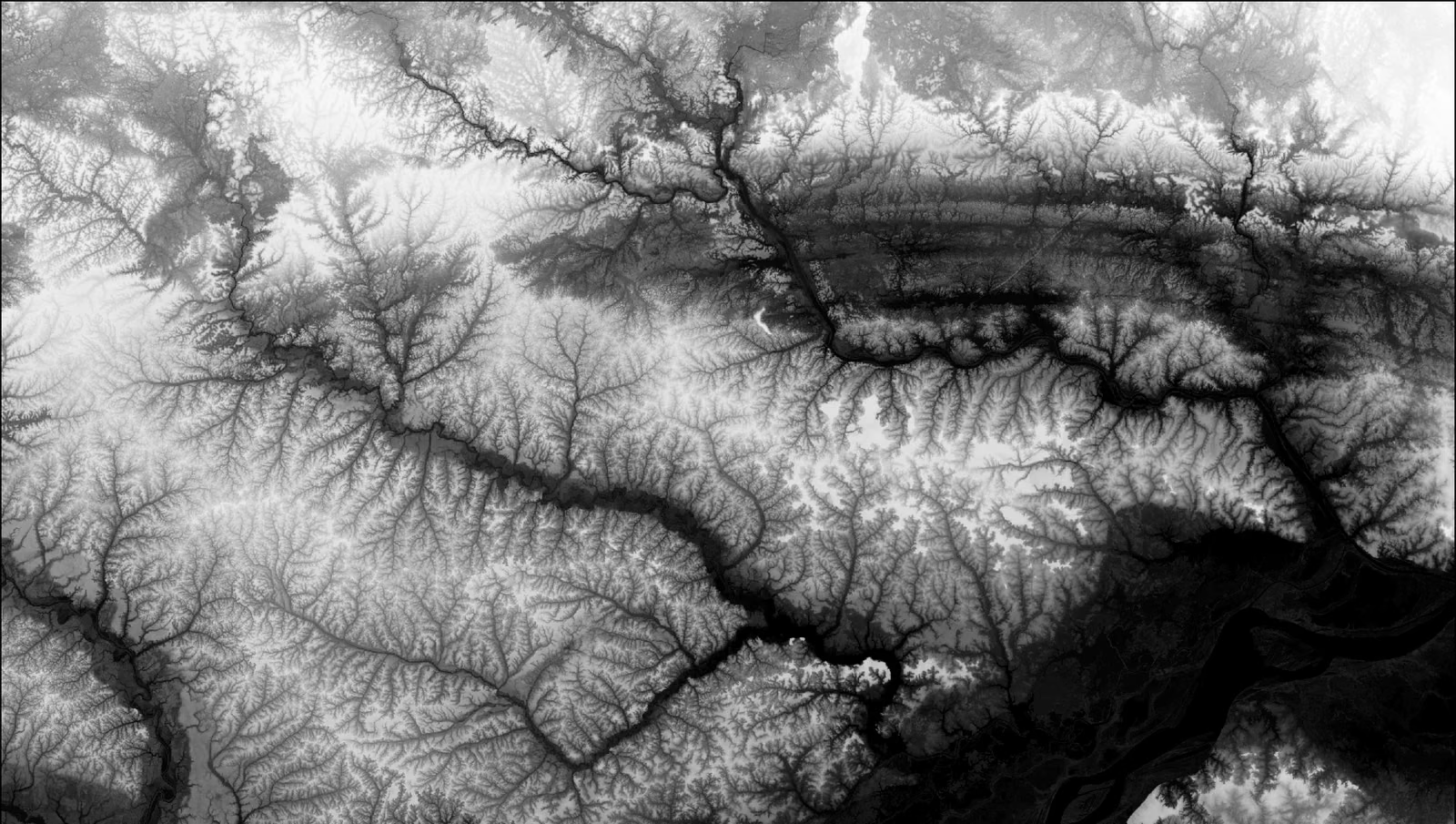
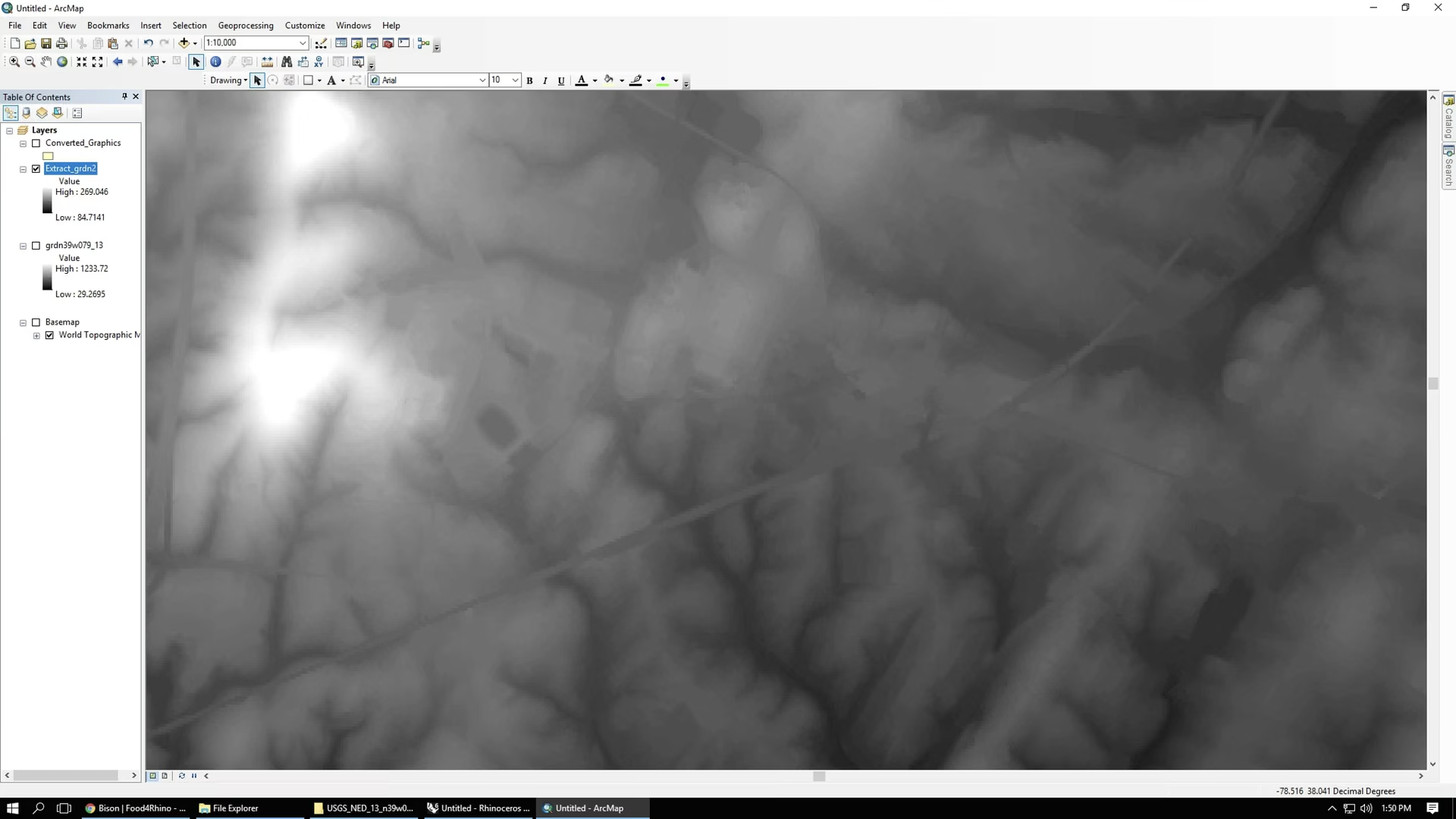
Digital elevation model
Digital elevation model detail
A digital elevation model rendered in grayscale
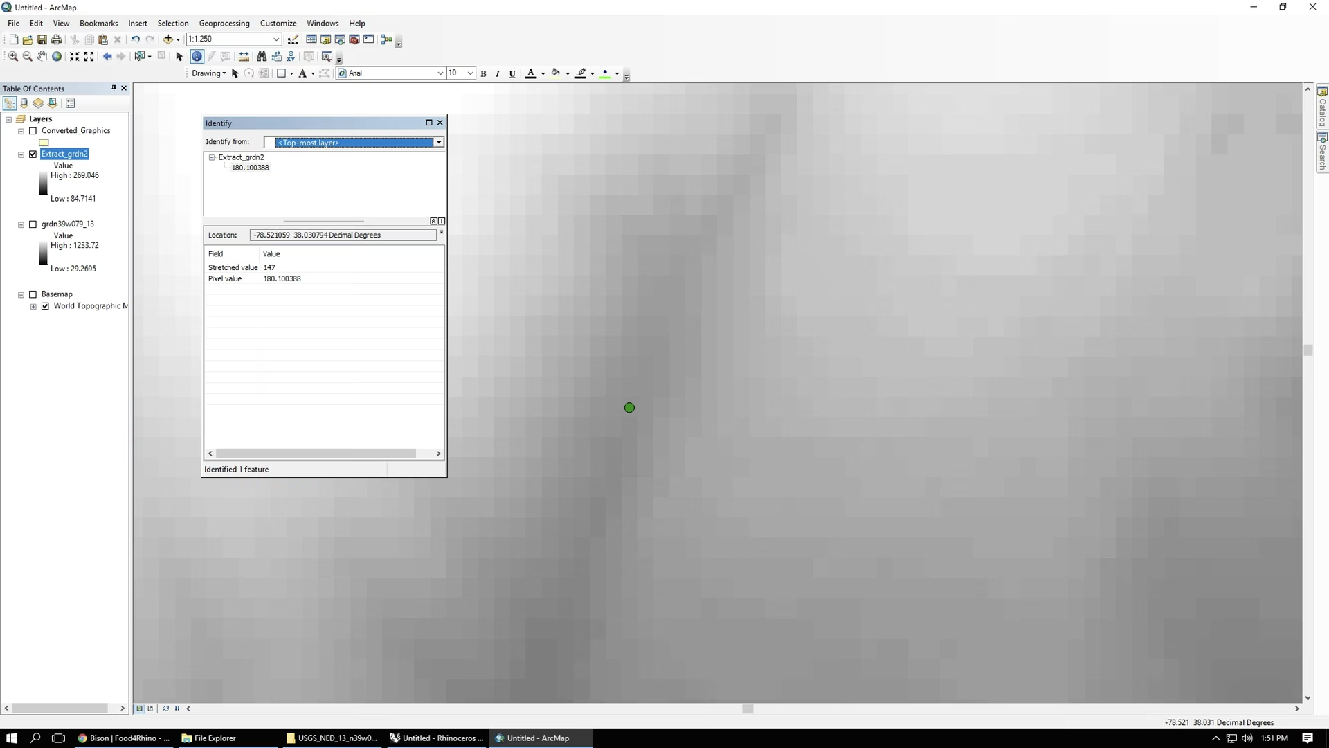
Raster terrain zoomed to reveal the grid of cell values
Map algebra / neighborhood operation on a raster grid
Part I

A map is an argument

Part II

From globe to grid

Part III

How space becomes data

Part IV

Analysis

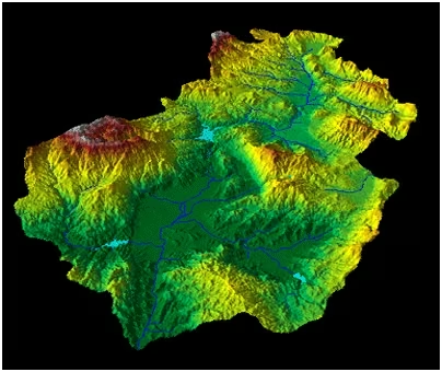
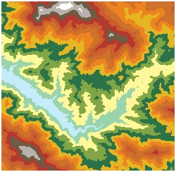
Colored digital elevation model
Elevation (DEM)
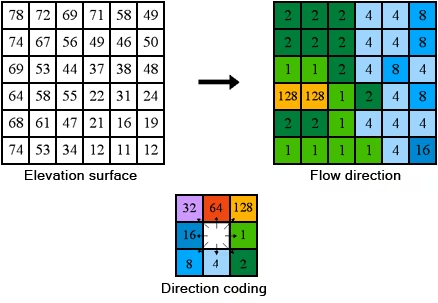
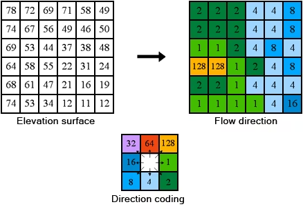
Elevation surface to flow direction, with the 8-direction coding scheme
Elevation → flow direction
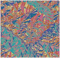
Flow direction raster derived from the DEM
Flow direction
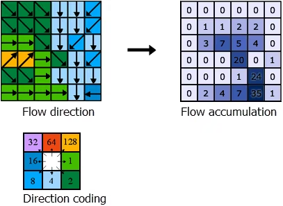
Flow direction grid to flow accumulation, with the 8-direction coding scheme
Flow direction → accumulation
Extracted stream network
Extracted stream
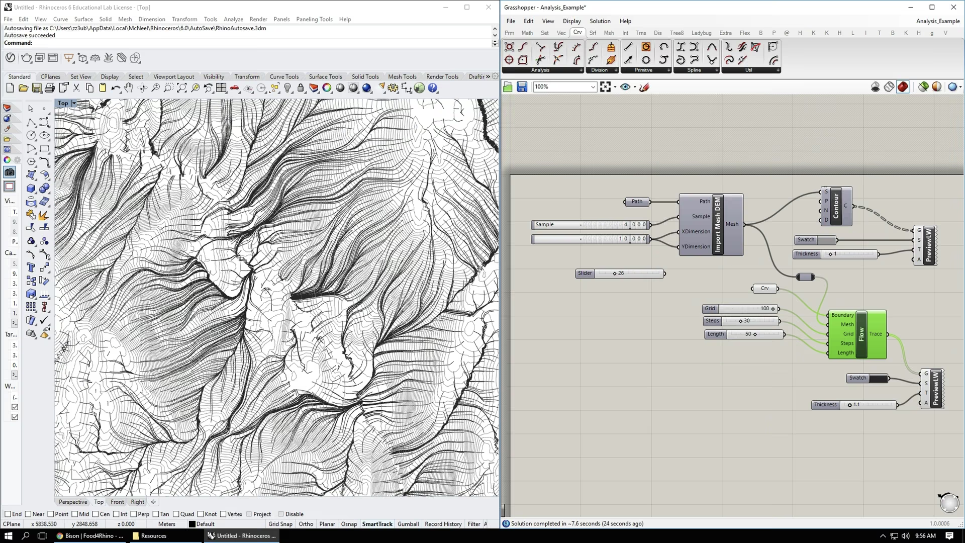
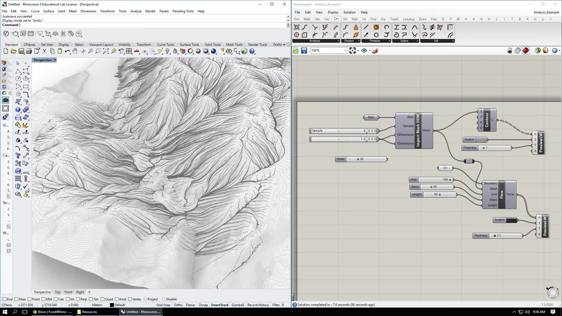
Terrain grid driving a parametric model in Rhino/Grasshopper
Terrain re-represented as mesh and contours in a Grasshopper definition
Worked example: elevation surface to flow direction, with the 8-direction coding scheme
# flow direction: for every cell, where does water leave?
DIR = {E:1, SE:2, S:4, SW:8, W:16, NW:32, N:64, NE:128}

for each cell (r, c) in DEM:
    center  = DEM[r][c]
    maxDrop = 0
    flow    = 0
    for each neighbor (nr, nc) around (r, c):   # the 3×3 box
        drop = (center - DEM[nr][nc]) / dist(nr, nc)
        if drop > maxDrop:
            maxDrop = drop
            flow    = DIR[ direction(nr, nc) ]
    FLOWDIR[r][c] = flow      # one of 8 codes — or 0 if a sink
“…to think is to test out, to operate, to transform.”
Maurice Merleau-Ponty · Eye and Mind · 1961
/ 26